Could Clinton Win Utah?

There’s been plenty of speculation this election season that Utahns’ distaste for Donald Trump might drive them so far as to “turn the state blue” in November, giving Hillary Clinton a plurality of the vote. I never took this speculation seriously, figuring that however much they dislike Trump, most Utahns are deeply loyal to the Republican Party and would therefore rationalize their way to hating Clinton even more.

But the fallout from Trump’s latest scandal has changed the landscape incredibly fast: his bragging in vulgar terms about habitually committing sexual assault has pushed many Utahns over the edge. Governor Herbert and several other prominent Utah Republicans have withdrawn their endorsements, and several who were on the fence have finally taken a stand against Trump, joining Mitt Romney, who has been a never-Trumper all along. Senator Hatch and my own Rep. Bishop are still supporting Trump, but they’re undoubtedly feeling a bit lonely at the moment. Most remarkable of all, the Deseret News has just published an editorial calling on Trump to drop out of the race, while expressing the hope that Congress will keep President Clinton in check.

Of course Utah won’t be the state that tips the balance of the Electoral College. But it’s still fun to consider whether Clinton could actually win Utah, so let’s take a look at the polling data. Here’s a screen capture from FiveThirtyEight.com, listing the nine Utah polls that weigh most heavily in that site’s Utah forecast:

The polls are listed in descending order by their FiveThirtyEight-assigned weights, based on the quality of the pollster, the sample size, and how recently the poll was conducted. The range of polling results is remarkably wide, but notice that the overall quality of the polling is poor: all of the polls are substandard in at least one of the three respects. Even the highest-weighted poll is by a pollster (Dan Jones) with only a C+ grade, and is now more than two weeks old. The highest-quality poll, conducted by SurveyUSA for the Salt Lake Tribune and the Hinckley Institute, is now four months old.

Nevertheless, FiveThirtyEight has combined all the Utah polls into a weighted average, then done some further processing to obtain a predicted most-likely outcome. Here’s a summary of the calculation:

The first four adjustments made to the polling average are small and, in my opinion, should be uncontroversial. One of these, the “trend line” adjustment, tries to update the older results based on trends in other states (and the nation as a whole) for which there is abundant recent polling. In principle, this adjustment should account for Clinton’s rise in the polls since the September 26 debate, up to but not including the events of the past two days.

But the adjusted polling average allocates only 81.9% of the vote to Clinton, Trump, and Johnson. The next step then assumes that nearly all of the remaining 18.1% will end up split evenly between Clinton and Trump, and here’s where I think the FiveThirtyEight model makes a Utah-specific error. The problem is Utah-based minor candidate Evan McMullin, who entered the race only two months ago yet seems to be polling almost as well as Johnson: 12% in the top-weighted Dan Jones poll, and 9% in the second-place PPP poll. It seems to me that if Johnson is allowed to retain his 12.6% share at this stage of the calculation, then McMullin should also retain his 10% or so.

FiveThirtyEight’s final adjustment is to mix in a prediction based not on polls but on a demographic regression model, which uses past voting patterns (broken down by region, race, religion, and educational level) to try to compensate for inadequate polling in states like Utah. (This is done even for the site’s “polls only” model, which is the one I’m working from.) But this adjustment could also be problematic, because of Utah’s (and Mormons’) peculiar affinity for Romney in 2012 and distaste for Trump in 2016.

So let’s back up to the “adjusted polling average” but tentatively give McMullin a share that’s 2% behind Johnson:

• Clinton 28.8%
• Trump 40.5%
• Johnson 12.6%
• McMullin 10.6%
• Other/undecided 7.5%

And now let’s ask how these numbers are likely to change over the next month, in light of the events of the last two days.

My guess is that a certain fraction of Trump’s 40.5% will follow Gov. Herbert’s lead and withdraw their support—some in direct reaction to the recent news and others because they now have “permission” from authorities they trust. Also, I doubt that Trump can now gain from any defections of Johnson, McMullin, or other/undecided voters. So unless there are further unexpected developments, it looks to me like Trump will end up with only 30% to 35% of the Utah vote.

Can Clinton’s share exceed this? If Trump gets only 30% then the answer is almost certainly yes: Clinton would then have to gain only a tiny fraction of the undecideds, Trump defectors, and perhaps defectors from minor candidates. If Trump can keep his vote share near 35% then it will be harder for Clinton, but still not out of the question. Let’s also remember that the percentages listed above are pretty uncertain, and you could make a case for discarding the weird outlying CVOTER International poll results; then Trump’s support would have already been below 40% even before the latest scandal.

Is there any chance that Johnson or McMullin could win? I think that would be a long shot, because they seem to be splitting the conservative anti-Trump vote so evenly. Only if one of them drops out, or otherwise implodes, would the other have a decent chance of surpassing Clinton.

The bottom line, in my opinion, is that Clinton is now a slight favorite to defeat Trump in Utah and carry the Beehive State. I say “slight” because of the large uncertainties in the past polling data, in the impact of the recent developments, and in what could still happen during the next 30 days. In any case, I can hardly wait to see what upcoming polls of Utah show, and to see how Utahns actually vote in such an extraordinary election.

Update, 16 Oct 2016: During the week since I wrote this article we’ve gotten three new Utah polls, and FiveThirtyEight has updated its Utah model to include Evan McMullin. Here’s their summary table of the polls that include McMullin, which are the only ones the model now uses:

The Y2 Analytics poll, first reported late on the night of the 11th, caused a flurry of excitement because it shows Clinton and Trump tied at only 26%. Equally remarkable is that McMullin is just behind at 22%, even though only 52% of respondents were aware of his candidacy. This result immediately made me question my earlier dismissal of McMullin’s chances. It also prompted articles covering the race in the New York Times, Washington Post, and FiveThirtyEight.

The subsequent polls from Monmouth and YouGov confirm that McMullin’s support is around 20%, but contradict the earlier indication that his gain has come entirely at the expense of Trump, whose support remains in the mid-30s. If these polls are a reasonably accurate predictor of the final results, then Trump will still win Utah by a safe margin.

After combining all six polls and making the minor adjustments described above, FiveThirtyEight now obtains the following “adjusted polling averages”:

• Clinton 24.1%
• Trump 33.8%
• Johnson 10.7%
• McMullin 19.4%
• Other/undecided 12.0%

Although Trump’s support has fallen about as much as I predicted a week ago, he remains comfortably ahead of Clinton because her support has also fallen somewhat (or at least is lower in polls that include McMullin). Could she or McMullin still win? Yes, because the uncertainty in these numbers is fairly large and the situation in Utah still seems pretty volatile. On the other hand, many Utahns will receive mail-in ballots during the coming week, so the clock is starting to run out. For what it’s worth, the PredictIt betting market, as translated by ElectionBettingOdds, currently has the odds of winning Utah at Trump 71.5%, Clinton 20.0%, and Other (presumably McMullin) 8.5%.

Update, 8 Nov 2016: Polls of Utah have been coming thick and fast over the last three weeks, but the picture hasn’t changed much over this time. Here’s another screen capture from FiveThirtyEight showing nearly all of the polls that include McMullin:

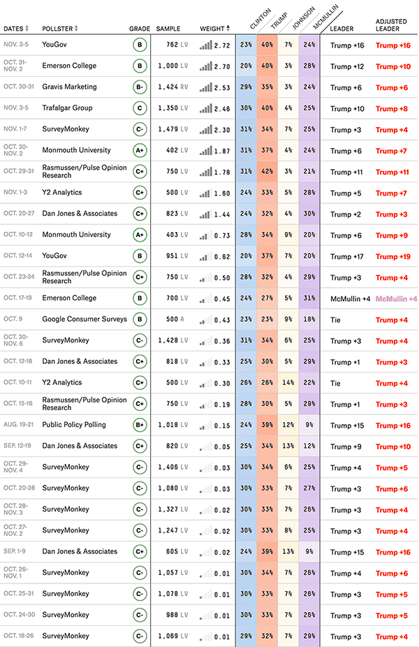
The general picture here is pretty clear: Trump is ahead in almost every poll, though there’s disagreement over whether his lead is by single or double digits. McMullin is the frontrunner in just one poll, and Clinton in none. Johnson has collapsed. Here are FiveThirtyEight’s averages and adjustments, to obtain its final prediction for the Utah presidential election:

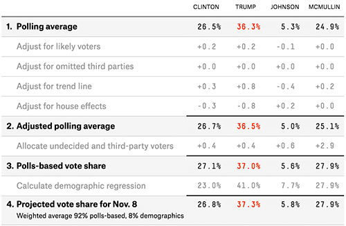
In the adjusted polling average, Trump comes out ahead of Clinton by nearly ten percentage points, while McMullin is behind Clinton by a point and a half. But then FiveThirtyEight assigns most of the remaining undecided voters to McMullin (presumably there’s a precedent for this), so McMullin ends up in second place in the final projection. The calculated win probabilities are Trump 82.9%, McMullin 13.5%, and Clinton 3.6%.

Meanwhile, Election Betting Odds has Trump at 87% likely to win, Clinton at 7%, and Other at 6%. Clinton’s higher odds here may reflect a recent report that she is ahead among early voters. It wouldn’t especially surprise me if Clinton beats her polls by a few points due to the early vote advantage, especially because many Utahns haven’t gotten used to Utah’s new mostly-by-mail voting system, and the number of physical polling locations has been greatly reduced since the last presidential election. Republicans who have hesitated this long because they’re unenthusiastic about all the candidates may have little motivation to find their polling locations and wait in the potentially long lines.

Still, it seems highly unlikely that either Clinton or McMullin will make up the roughly ten-point polling deficit to catch Trump, who will probably win Utah with less than 40% of the vote.

Just as Trump’s potential national victory says a lot about the state of American politics, so also his ability to win Utah tells us that our state isn’t as different as many would like to believe. Although many prominent Utah politicians have denounced Trump, Reps. Chaffetz and Stewart ultimately backtracked and said they would vote for him anyway. Governor Herbert and Mitt Romney have remained silent about whom they’re voting for. (A McMullin endorsement from either of them, which I was half expecting four weeks ago, might have put McMullin in the lead.) The bottom line is that even though most Utahns fully understand that Trump is a lying, bigoted, asshole who’s absolutely unqualified for the job, their allegiance to the Republican Party drives them to dislike Clinton even more. Many Utahns will explain that at least Trump will (he says) appoint anti-abortion justices to the Supreme Court. Few of them, I suppose, have carefully thought through the risks that America and the world will face if Trump actually wins.

Update, 19 January 2017: Before the inauguration of President Trump I suppose I should finish this saga with the actual Utah election results:

• Trump 45.5%
• Clinton 27.5%
• McMullin 21.5%
• Johnson 3.5%
• Others 2.0%

Comparing to the final FiveThirtyEight polling averages above, we see that not only did essentially all of the undecided voters apparently end up voting for Trump, but he also picked up a fair number of McMullin and Johnson defectors in the final days before the vote. This result fits in nicely with the conventional wisdom about what happened in the decisive swing states, with the further complication that a larger percentage of Utah voters was up for grabs. Of course, it’s also possible that there was a systematic polling error in Utah, such as an under-sampling of white voters without college degrees. In any case, I was obviously wrong to predict that Trump would end up with under 40% of the vote. As for Clinton, she did over-perform her polls as I more or less predicted, but only by about a point.

Despite my poor numerical predictions, I think the overall tone of my final election-day paragraph holds up pretty well. Of course the important question now is what will happen during Trump’s presidency. The nation is headed into uncharted territory, with a vast range of possible outcomes ranging from reasonably normal to absolutely catastrophic. I don’t see how anyone could possibly predict what will happen.

A Year of Solar Data

My solar panels were installed in August of last year, and two months later I reported on how they were performing. Now, after a full year of operation, it’s time for a more comprehensive report.

The bottom line is that the panels produced a little less electrical energy than the installer predicted, but still quite a bit more than I used over the course of the year. Here’s a diagram showing the overall energy flows:

Here and throughout this article I’ll present data from the year that began on 1 September 2015 and ended on 31 August 2016. During that time the panels produced 1558 kilowatt-hours (kWh) of electrical energy, and I used 349 kWh of that energy directly. The other 1209 kWh went onto the grid for my neighbors to use. But I also pulled 813 kWh of energy off the grid, at night and at other times when I needed more power than the panels were producing. My total home usage from both the panels and the grid was 1162 kWh. (I got the solar production amount from my Enphase solar monitoring system, and the amounts going to and from the grid by reading my electric meter. From these three numbers I calculated the other two.)

Because I used less energy than my panels produced, I’ve paid no usage charges on my electric bills since the system was installed; I pay only the monthly minimum charges, which come to about $9.00 per month including taxes. Under Utah’s net-metering policy (which could change in the future), each kWh that I push onto the grid can offset the cost of a kWh that I pull off of the grid at some other time. But I don’t get to make a profit from the 396 kWh excess that I pushed onto the grid over the course of the year; that was effectively a donation to Rocky Mountain Power, worth about $40 at retail rates.

Monthly and daily details

So much for the yearly totals. But the picture varies quite a bit with the seasons, as shown in this graph of my panels’ monthly output:

The total energy generated in July (165 kWh) was twice as much as in January (81 kWh), with a pretty steady seasonal rise and fall in between. On the other hand, my installer estimated significantly higher production in winter and spring, plotted on the graph as green squares. (I get a similar over-estimate of the winter and spring production, relative to summer and fall, when I use the NREL PVWatts calculator, with weather data from the Ogden airport. So maybe my location is cloudier than the airport, and/or maybe last winter was cloudier than the 30-year average that the calculator uses.) The actual annual production of 1558 kWh was 91% of the estimated total of 1713 kWh. (An earlier, less formal estimate from the installer was 1657 kWh for the year, and not broken down by month; my annual production was 94% of that estimate.)

You might think the factor-of-2 seasonal variation in my solar energy production was a direct result of the varying length of the days and/or the varying solar angles. In fact, however, it was mostly due to varying amounts of cloud cover. You can see this in a plot of the daily energy generated:

The energy output on sunny days varied only a little with the seasons, and was actually lowest in the summer. But summer days in northern Utah are consistently sunny, whereas a full day of sunshine can be uncommon in mid-winter. Incidentally, my best day of all was February 23 (6.7 kWh), while my worst day was January 30 (0.0 kWh, because it snowed throughout the day).

Although the seasonal variations among sunny days are relatively small, they’re still interesting. The output drops off in mid-winter because the days are shorter, and also because the mountains block the early morning sunlight. On the other hand, the output drops off in the summer because of the steep angle of my roof. The panels face the noon sun almost directly throughout the fall and winter, but they face about 37 degrees too low for the mid-summer noon sun, reducing the amount of solar power they receive by about 20% (because the cosine of 37° is 0.8). The following plot shows all these effects:

Notice that the vertical axis on this plot is power, or the rate of energy production. To get the total energy generated you need to multiply the power by the time elapsed, which is equivalent to calculating the area under the graph. As you can see, the June graph is lowest at mid-day but extends farther into the early morning and late afternoon, while the December graph is highest but narrowest. The total energy (area) is largest for the March graph. The asymmetry in the December graph, and in the lowest part of the March graph, is from the mountains blocking the rising sun. The smooth “shoulders” on either side come from the shadow of the pointy gable in the middle of my roof.

With all of these effects in mind, as well as the day-to-day variations in cloud cover, let me now show all of my solar data for the year in a single image. Here the day of the year is plotted from top to bottom, and the time of day from left to right. The power level in watts is represented by color, with brighter colors indicating higher power levels:

In the upper-left portion of this image you can more or less see the shape of the mountains, with a reflection at the winter solstice. The dark stripes are cloudy days, with the exception of a power outage during the wind storm of May 1 (that’s right—a standard grid-connected photovoltaic system produces no power when the grid goes out). Subtle astronomical effects cause some further asymmetries from which, with enough analysis, you could probably extract the shape of the analemma.

Details aside, the big picture is that the steepness of my roof is almost ideal for the winter months. It even ensures that snow slides off the panels as soon as the sun comes out. But the steep angle hurts my solar production more in the summer than it helps in the winter, mostly because so many winter days are cloudy anyway.

Effect of temperature

Looking back at the previous graph for the three sunny days in different seasons, you might have noticed that the noon power level drops from winter to summer by more than the 20% predicted by the solar geometry. The discrepancy on any particular day could be due to variable amounts of haze, but there’s another important effect: temperature.

To isolate the effect of temperature, I took the noon power level for every day of the year and divided it by the (approximate) cosine-theta geometrical factor to get what the power would have been if the panels were directly facing the sun. Then I plotted this adjusted power level vs. the ambient temperature (obtained from Ogden-area weather reports) to get the following graph:

The data points cluster along a line or curve with a negative slope, confirming that the panels produce less power at higher temperatures. Very roughly, it appears that the power output is about 15% less at 90°F than at 20°F. For comparison, the data sheet for the solar panels indicates that the power should drop by 0.43% for each temperature increase of 1 degree Celsius, or about 17% for an increase of 70°F. But this specification is in terms of the temperature of the panels, which I wouldn’t expect to vary by the same amount as the ambient temperature.

(In the preceding plot, the outlying data points below the cluster are from days when clouds reduced the solar intensity; most such points lie below the range shown in the graph. I’m pretty sure that the outliers above the cluster are from partly cloudy days when the panels were getting both direct sunlight and some reflected light from nearby clouds.)

Electricity usage

Now let’s look at the seasonal variation in my home electricity usage, compared to the solar panels’ output. Here’s a graph of the monthly data, with the solar data now plotted as blue squares and the usage plotted as columns, divided into direct-from-solar usage and from-the-grid usage:

Unfortunately, my electrical usage peaks in mid-winter, when the solar production is at a minimum! But even during the bulk of the year when the solar production exceeds my total use, well over half of the electricity I use comes off the grid, not off the panels.

The good news is that I’ve actually reduced my total electricity use by about 15% since the panels were installed. I did this through several small changes: running the furnace less when I was away from home; cooling my house in the summer with a super-efficient whole house fan instead of smaller fans sitting in windows; and unplugging an old computer and a portable “boom box” stereo that were drawing a few watts even when turned off. I’m still using more electricity than I did a decade ago, when I had no home internet service and no hard-wired smoke detectors. But if you look just at what I’m using off the grid, it’s slightly lower even than back in those simpler times. Here’s an updated plot of my average daily usage during every month since I bought my house 18 years ago (as explained more fully in this article from last year):

What would it take to live off the grid?

I’ve repeatedly emphasized the electrical energy that I continue to draw from the grid, because I want readers to understand that virtually all of the solar panels being installed these days are part of the electrical grid—not an alternative to it. Even though my panels generate more electrical energy than I use over the course of a year, they will not function without a grid connection and of course they generate no power at all during most of the times when I need it.

But what would it take to live off the grid entirely? The most common approach is to combine an array of solar panels with a bank of batteries, which store energy for later use when the sun isn’t shining. For example, there’s been a lot of talk recently about the new Tesla Powerwall battery, which stores 6.4 kWh of energy—enough to power my home for about two days of average use. A Tesla Powerwall sells for $3000, which is somewhat more than the net cost (after tax credits) of my solar panels. If I were to make that further investment, could I cut the cord and live off the grid?

To answer this question, I combined my daily solar generation data with a data set of nightly readings of my electric meter. (The latter data set is imperfect due to inconsistent reading times, missed readings when I was away, and round-off errors, but day-to-day errors cancel out over longer time periods so it should give the right picture overall.) I then calculated what the charge level of my hypothetical Tesla Powerwall would be at around sunset on each day, and plotted the result:

For most of the year the battery would hold more than enough energy to get through the nights, but in this simulation there were 42 evenings in the late fall and winter when the level dropped to zero, and several more evenings when it dropped low enough that it would surely be empty by morning. Simply getting a Tesla Powerwall is not enough to enable me, or most other households with solar panels, to disconnect from the grid.

What if I added a second Tesla battery? Unfortunately, that would reduce the number of zero-charge nights by only eight, from 42 to 34. In fact, it would take thirteen Tesla batteries, in this simulation, to completely eliminate zero-charge nights, because there is a period of a few weeks during mid-winter when the average output of my solar panels is barely over half what I’m using.

The better solution, therefore, would be to add more solar panels. For example, if I were to double the size of my solar array and install two Tesla Powerwalls, then the simulation predicts that I would run out of electricity just one night during the year. Of course this scenario is still extremely wasteful, because I’d be using less than half the capacity of the panels and only a small fraction of the capacity of the batteries during most of the year. That’s why people who actually live off the grid tend to have backup generators that run on chemical fuels, and don’t rely on electricity for most of their heating or cooking.

Similar calculations would apply to our society as a whole. A massive investment in both solar panels and batteries could conceivably get us to the point where most of our electricity, for most of the year, is coming from the sun. But it will never be economical to get that “most” up to 100%, because so much over-building would be needed to get through periods of cloudy weather, and it will be much less expensive to use other energy sources at those times.

Who Needs Air Conditioning?

As I write these words the temperature outside is 91 degrees Fahrenheit, and the August sun has been beating down on my house for several hours, yet the inside temperature is an extremely comfortable 76.

That would hardly be remarkable in this day and age, except that my house has no air conditioning. I don’t even have an evaporative (“swamp”) cooler, which is a great alternative to air conditioning in the arid interior West.

Instead I rely on another benefit of Utah’s low humidity: the nights are almost always quite cool, so I can open windows and run fans to cool off the house at night. Then I shut everything up in the morning as the sun is rising over the mountains, and rely on my house’s thermal inertia to keep it comfortable for most or all of the day.

Of course, this old-fashioned, low-tech way of keeping cool is technically inferior to the modern method of just leaving the thermostat set at your preferred temperature. For one thing, opening and closing windows is hard work! Also, during the course of a typical summer day and night, while the outdoor temperature swings up and down by 30°F, I experience indoor temperature swings of as much as 15°F. Here’s some data (logged by my smart thermostat) from a recent two-week period:

The indoor temperature swings mean that I might need to wear a sweatshirt in the early morning, take it off after a couple of hours, and perhaps sit in front of a small fan on the hottest late afternoons, when it climbs above 85°F. When I go to bed at night I rarely want more than a sheet over me, but after a few hours, as the house continues to cool, I usually reach for the blankets.

Maybe I’m a fanatic for happily enduring these needless, though minor, discomforts. But I can honestly say that a bit of discomfort makes me feel much more alive and connected to the surrounding world—in the same way as riding a bicycle instead of driving a car. As the late, great Tom Magliozzi said, “I mean, before you know it, you're going to spend plenty of time sealed up in a box anyway, right?”

And, of course, using windows and fans for “air conditioning” saves massive amounts of energy, greenhouse gas emissions, and money.

“But wait!,” you ask, “Don’t you have solar panels on your roof?” Indeed I do, but I would need at least twice as many of them to offset the electricity needed by a modest central air conditioning system in regular use. Also, there’s a time lag of several hours between peak solar generation (high noon) and peak air conditioner use (late afternoon), so solar panels by themselves cannot meet all of America’s air conditioning demand. Yes, we could envision massively expensive battery storage systems, but it’s vastly more practical, at least here in Utah, to just forgo the technology and open the windows at night.

Let me say a bit more about fans. Until this summer my arsenal included a basic 12-inch oscillating fan, which I typically placed on a bedroom windowsill at night, and a similarly inexpensive plastic window fan, containing two 7-inch fan units, which I typically placed in the kitchen window. At their highest speeds these fans use 40 and 110 watts, respectively, and they do a pretty good, but not great, job of cooling off the house. The window fan is pretty noisy, so I would usually close a door between it and the bedroom.

In June, however, I invested some money in a major upgrade: an AirScape 2.5e whole house fan.

A whole house fan is mounted in the attic above a hole in the ceiling, so it pulls air upward into the attic from the living space while pushing the hot air out of the attic. You run it only at night, with your windows open, so cool air can come in the windows to replace the air pulled upward by the fan. You can choose which room(s) to cool off most quickly, simply by choosing which window(s) to open.

Some whole house fans can be awfully loud, but AirScape is the Rolls Royce of whole house fan manufacturers, and the model 2.5e is extremely quiet—especially toward the lower range of its five speed settings. The fan itself is suspended from chains a few feet above the attic floor, at the end of a seven-foot flexible duct that provides acoustic isolation. At the other end of the duct, immediately above the opening in the ceiling, is a box containing motorized damper doors. Here are some photos of the installed fan in the attic, the view looking up at the ceiling and the damper doors, and the wall switch (mounted next to my Ecobee thermostat):

The motorized damper doors, in place of a simpler and less expensive back-draft damper, provide good insulation when closed and allow the fan to run at very low speeds, producing only the gentlest breeze. I usually run my fan all night long, choosing the speed based on how hot the house has gotten by evening.

The AirScape 2.5e is also extremely efficient: it draws only 25 watts on the lowest setting, and 200 watts on the highest (which I rarely use). Even on the lowest setting it’s about as effective as my two old inexpensive fans, which together use 150 watts and make much more noise. For comparison, a small central air conditioning system would use about 2500 watts while running.

As if the motorized damper doors aren’t already fancy enough, these AirScape fans can now also be connected to your home network router and then controlled through a smartphone app. This technological sophistication seems a little excessive to me, but the app, unlike the wall switch, tells you the current speed setting and even displays the attic temperature. You can only use it from home—not over the internet—but there would be little point to controlling it remotely unless you also had remote-control windows. Actually I wish AirScape would make a lower-tech damper assembly that you just open and close by hand with a lever, avoiding the complication and expense of all the electronics. This would also eliminate the continuous 8-watt electrical power draw from the electronics, even when the fan is turned off. (To avoid this small energy waste I’ll switch the fan off at the circuit breaker at the end of the summer.)

Of course, Rolls Royces don’t come cheap. With shipping I paid a little over $1500 for my AirScape 2.5e, and then I paid my favorite local HVAC contractor a few hundred dollars more to install it. Even so, it cost less than any central air conditioning system I’ve ever heard of—and you could easily install the fan yourself if you have a helper and the right tools. But I don’t mind spending this money on a long-term improvement to my home, especially when I’m supporting a good company that makes such a useful product. AirScape fans are designed and made in Medford, Oregon.

Not every house is suitable for a whole house fan. It won’t be nearly as effective in a location where summer nights are warm. Your attic must be well ventilated, so the fan can push the air out (see the AirScape web site for detailed ventilation requirements). And for ducted models like the 2.5e, you need a reasonable amount of vertical space in the attic. But if your house meets these criteria and you have the money to invest, then I highly recommend this elegant alternative to air conditioning.

The Ecobee Smart Thermostat: A Data Junkie’s Dream

In an attempt to reduce my heating bills and carbon footprint, last September I installed an Ecobee 3 smart thermostat.

Now, after using it through a full heating season and analyzing the results, I can report that it accomplished everything I hoped.

Should you buy one too? That depends.

Why the Ecobee?

The idea behind a “smart” thermostat is to gather a whole bunch of data (past temperatures and settings, furnace and AC run times, outdoor weather, and times when you’re home and awake), then use this data to anticipate your heating and cooling needs and to keep you comfortable, automatically, without wasting energy. If you want a thermostat that does this then you can consult any number of online reviews for advice.

I don’t want my thermostat to set itself automatically. I’m fully capable of setting it myself, thank you very much, and I stubbornly cling to the notion that I’m still smarter than any thermostat.

But I decided to get a smart thermostat anyway, because I wanted the ability to remotely monitor the temperature in my house over the internet, and to remotely adjust the setting from time to time. Also, I wanted to get my hands on all that data. As usual, I take my mantra from Mr. Money Mustache: Measure everything, then get angry at waste!

The most popular smart thermostat is the Nest, but for my purpose it has a fatal flaw: They don’t let you download the data! You can view some daily summary data over the internet, and they send you monthly summaries by email, but the manufacturer has decided that you’re not even allowed to see the full minute-by-minute temperature and operation data, much less download it.

The Ecobee folks, on the other hand, treat their customers with respect. Through their web interface you can view a detailed chart of what’s happening in your house, and with a few clicks you can download the data as a CSV file for analysis in a spreadsheet or other software.

That feature was enough to earn my business, so I went ahead and ordered an Ecobee, directly from the manufacturer. The price was $249, but I got a $100 rebate from my gas company. Installation was easy, although there can be complications depending on how your existing system is wired. With a couple of taps on the touch screen I configured it for fully manual operation.

My house has no air conditioning, so during the summer I use the Ecobee only as a remote-monitoring and data-logging device. It does, of course, use some electricity to accomplish these things: about 7 watts of continuous power, which adds up to 60 kilowatt-hours (about $6 worth here in Utah) of electrical energy per year. It also requires a continuously operating internet connection and wifi router.

One unique feature of the Ecobee 3 is that it comes with a wireless, battery-powered external sensor that you can use to monitor the temperature in another room, away from the thermostat. Their advertising suggests that this is almost as good as being able to heat different parts of your house independently, but of course that’s not the case; you merely have the flexibility to control the heat based on the temperature at one or another location. I put the external sensor in my basement laundry room, so I could make sure the pipes wouldn’t freeze when I was away during the winter. (Being a data junkie, I eventually purchased two more external sensors, for another $79, so I could also monitor the temperature in my living room and bedroom.)

How I cut my gas use by 35% [see update below]

As it turned out, that external sensor in the basement is what saved me the most money. I was away from home quite a bit during the winter of 2015-16, and at those times I aggressively set the thermostat down, letting the temperature drop to 48 F upstairs and 40 F in the basement. Without the sensor next to the water pipes, and the ability to remotely monitor it and make adjustments if needed, I never would have taken the risk of turning the thermostat so low.

To put my savings in perspective, here’s a plot of my annual natural gas use ever since I bought my house in 1998:

The total for 2015-16 was 18.4 decatherms (MBtu), or 35% less than my average use from 2004 through 2015. When you consider that some of that (about 4 decatherms, I think) is for my hot water heater, the reduction is even more impressive. Gas is cheap here in Utah—about $8 per decatherm—so I saved only about $80 over the season, and it’ll take another year before the thermostat nominally pays for itself. On the other hand, not all of the reduction was a direct effect of the smart thermostat: my motivation to save energy was probably at an all-time high, and it’s possible that the winter was a little warmer than average [see update below].

Getting the detailed data

And what about the detailed thermostat data? Here, to start with, is a screen capture showing what you can view through the Ecobee web interface:

The orange graph is the thermostat setting; the white graph is the temperature at the thermostat; the green graph is the outdoor temperature (obtained from public weather data for my local area, so it’s not literally the temperature right outside my house); and the orange bands at the top show when the furnace was running. On this particular day I kept the thermostat at 64 degrees when I was home, but set it down to 58 when I was at work. The furnace cycled on and off seven times between midnight and 8 am, didn’t run at all while I was away, ran for more than a half hour to warm the house up when I returned, and then cycled on and off four more times before midnight.

This web interface to the data is a wonderful thing, but I find it a little clunky and hope they’ll make some improvements in the future. Although you can scroll through the entire time period since your thermostat was installed, you can’t zoom out to view more than 24 hours of data at a time. Updating the graph with new incoming data requires multiple clicks and a delay of about 10 seconds. The graph always omits the most recent hour or so, and it won’t show the separate data from all your sensors, even though you can view all the current readings on a different web page.

To get a more comprehensive picture you need to download the data and plot it up yourself. Fortunately, the download process is easy and fast. As I mentioned above, you get a CSV file that you can open in a spreadsheet. The file contains a row for every five-minute time interval, and each row contains 20 or more data fields: date, time, thermostat settings, heating/AC/fan activity, outdoor temperature and wind speed, and, for the thermostat itself and each external sensor, the temperature and whether the motion detector was activated. You can download up to a month’s worth of data (more than 8000 rows) at a time.

The ways of plotting up all this data are endless. Here, for example, is a plot of my temperature data for the month of July. Can you guess which week I was out of town?

Thermal properties of my house

One of my goals in obtaining all this data was to measure the thermal properties of my house. To do this I focused on the six-month heating season from November through April, and selected eight-hour-long periods at night (to avoid solar heating) when either the furnace was holding the indoor temperature steady, or the furnace didn’t run at all. (I didn’t use data from nights when neither of these conditions was met for eight consecutive hours.)

Working with the steady-temperature data, I used the furnace running time to calculate the rate at which the furnace had to supply heat to the house, to maintain the steady temperature. To calculate the heat rate I had to know that the furnace is rated to use 75,000 Btu per hour, at an efficiency of 92%; I’ve checked the Btu/hr value by reading my gas meter, but I have no good way to check the efficiency. Here is a plot showing the heating rate as a function of the average temperature difference between inside and outside:

You can immediately see from this plot that my 75,000 Btu/hr furnace (69,000 Btu/hr when you factor in the 92% efficiency) is much more powerful than necessary. Even on the coldest nights it needed to put out only about 14,000 Btu/hr to maintain a steady indoor temperature, so it was running only about one fifth of the time. Extrapolating, I conclude that my furnace could maintain a steady indoor temperature even if the outdoor temperature were as much as 200 degrees lower than indoors! How’s that for over-engineering?

A linear fit to the plotted data gives a slope of approximately 344 Btu per hour per degree Fahrenheit, meaning that for each additional degree in the temperature difference, the furnace had to supply additional heat at a rate of 344 Btu/hr. Of course that heat must also be escaping from the house (through the walls, windows, ceiling, and foundation) at the same rate, because the indoor temperature wasn’t changing. The value 344 Btu/hr/°F is therefore what is called the thermal conductance of the exterior envelope of my house.

There’s quite a bit of scatter in the data, so this measured conductance is somewhat uncertain. The standard error in the best-fit slope is only 6.4%, but when I plot subsets of the data (chosen by time of year or thermostat setting) I get a much wider range of values, so I would put the uncertainty very roughly at 20%.

You can also see from the plot that a best-fit line does not go through the origin; in fact the vertical intercept is at −2800 Btu/hr, with a rather large uncertainty (perhaps 40%). This means that on a typical winter night, heat from some other source must be entering my house at a rate of roughly 2800 Btu/hr, or about 800 watts. Some of that is from the refrigerator, electric blanket, and human bodies, but after slicing and dicing the data I’m convinced that there’s also a contribution from underground heat coming in through the basement floor and foundation.

In principle, you can calculate the thermal conductance of a house without making any temperature measurements at all. You just need to know the sizes and thermal conductivities (R values) of the components of the exterior envelope. Add the R values for each layer of a given component (e.g., plaster, wood, brick, and air films for my uninsulated walls), then divide this total R value into the surface area to get that component’s contribution to the conductance. I had never before done this calculation for my house, because there’s a lot of guess-work involved and I had no good way to check the answer. But now I have done the calculation, and amazingly, I obtained a total conductance of 374 Btu/hr/°F, within ten percent of the measured value! The pie chart shows a breakdown of how each major component of my house’s envelope contributes to this calculated total.

The ceiling contribution is small because it’s the only place where my 81-year-old house has at least a little bit of insulation. Of course, these fractional contributions could still be pretty inaccurate. But I now have enough confidence in my calculations to start considering whether I should try to add insulation to my exterior walls and foundation.

By the way, people sometimes say that homeowners should focus on air infiltration as a major source of heat loss. That may be true for some homes, but I’ve always been skeptical in my own case. My calculations justify this skepticism because I was able to account for more than 100% of my house’s measured heat loss through conductance estimates alone, completely ignoring infiltration.

Meanwhile, as mentioned above, I’ve also looked at data from winter nights when the furnace didn’t run at all—so the indoor temperature dropped steadily. Here is a plot of the rate of temperature decrease as a function of the average temperature difference between inside and outside:

The slope of this graph is minus the thermal conductance divided by the effective heat capacity of the interior of my house. (So a high thermal conductance makes the graph steeper, because heat escapes faster, while a high heat capacity makes it shallower, because there’s more energy that needs to escape in order for the temperature to drop by a given amount.) The best-fit slope is −0.023 degrees per hour, per degree (or simply inverse hours if you prefer). Dividing this into the previously measured conductance of 344 Btu/hr/°F gives a heat capacity of approximately 15,000 Btu/°F. That’s equivalent to the heat capacity of 15,000 pints of water, or 1800 gallons, or enough to fill my bathtub up to the brim 26 times. So filling the bathtub wouldn’t make much of a dent in the total heat capacity!

An alternative way to estimate the heat capacity is simply to measure how long it takes the furnace to warm the house up after adjusting the thermostat upward. For example, on one winter evening it took my furnace two hours to warm the house by 14 degrees Fahrenheit. The furnace supplied 138,000 Btu of heat over that time, so the estimated heat capacity would be (138,000 Btu)/(14°F) = 10,000 Btu/°F. The effective heat capacity is smaller over this relatively short time period, because less of the house is actually being warmed up by the full amount.

In principle I could try to calculate a theoretical heat capacity, by adding up all the contributions of the materials and contents of my house. It would be interesting to know roughly what percentage comes from wood, plaster, concrete, and so on. But making reasonably accurate estimates would be quite a bit of work, so I’ll put that off to another day.

The more useful thing to know is that even on a very cold night (bottom-right corner of the graph), my house cools down at a rate of less than a degree Fahrenheit per hour. This means that setting the thermostat down for, say, eight hours at a time saves only a small amount of energy, because the average indoor temperature over that time will be no more than two or three degrees lower. This average drop is what matters, because it determines how much less heat the house loses to the outdoors—and therefore how much less heat the furnace must replace. Any further energy savings from not running the furnace during this time will be offset when you run it to heat the house back up afterwards. (You can see all this vividly in the screen-capture image above.)

So how did I save huge amounts of energy, cutting my gas bill by 35%? Partly by setting the thermostat somewhat lower even when I was home, but mostly by setting it way down when I was away for 24 hours at a time or longer. If your house is never unoccupied for more than half a day at a time, then you shouldn’t expect dramatic winter energy savings from a smart thermostat. Summer might be another matter if you use air conditioning, but I wouldn’t know. And if you own a vacation home that’s unoccupied for half the winter, then install a smart thermostat in it immediately!

Update, July 2019

Honesty compels me to report that over the last three years I’ve failed to keep my gas use as low as it was during 2015-16. Here is an updated chart:

Over these last three years my annual gas use has averaged 23.6 decatherms, which is only 16% less (not 35% less!) than the average from 2004 through 2015 (before I installed the Ecobee thermostat). The most recent winter was the coldest of these three, so I’m not too worried about a continuing upward trend in gas use as the chart might suggest. Instead I think I’ve reached a new normal, after the anomalous one-time low during 2015-16.

The direct carbon emissions from burning 23.6 decatherms of natural gas come to 1.25 metric tons (2760 pounds), so this contribution to my personal carbon footprint is somewhat larger than any one of the contributions from electricity use, driving, or flying.

Ivory Tower

Thanks to the Utah Film Center and all its generous supporters, I just saw a free screening of Ivory Tower, the 2014 documentary about the problems facing American higher education.

For the most part I thought the film was excellent. It focused on the crisis of rising tuition and student loan debt, and touched on most of the reasons why this crisis has arisen: growing enrollments, shrinking state subsidies, and increased overhead costs for bloated administrations and frivolous amenities. The film also explored a variety of innovative variations on higher education, ranging from massive open online courses to the tiny Deep Springs College. It came down heavily against impersonal, one-size-fits-all solutions, and emphasized the importance of one-on-one human interaction.

The film fell short, though, in its inadequate attention to profit motives. It didn’t even mention the for-profit college sector, which has played a disproportionate role in the student debt crisis. It seemed to blame the federal government for pushing loans on students, when in fact it’s private banks and investors who are profiting from those loans. And although it highlighted the for-profit MOOC startups Udacity and Coursera (and the much-publicized collaboration between Udacity and San Jose State University), it failed to mention the lower-profile infiltration of software for canned courses that’s coming from traditional textbook publishers.

To get to the bottom of a scandal, you need to follow the money.